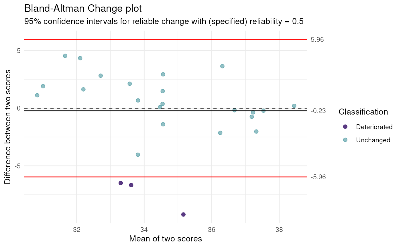
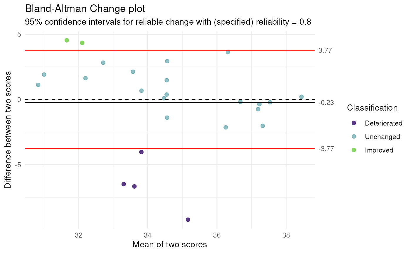
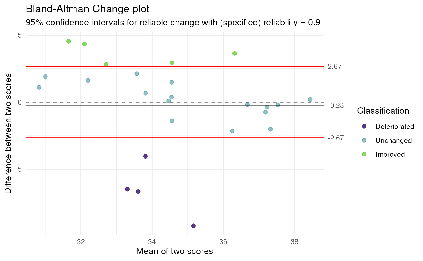
Bland-Altman Change plot

BAC_plot(
  data,
  cols = names(data),
  reliability = NULL,
  pointSize = 2,
  deterioratedColor = "#482576E6",
  unchangedColor = "#25848E80",
  improvedColor = "#7AD151E6",
  zeroLineColor = "black",
  zeroLineType = "dashed",
  ciLineColor = "red",
  ciLineType = "solid",
  conf.level = 0.95,
  theme = ggplot2::theme_minimal(),
  ignoreBias = FALSE,
  iccFromPsych = FALSE,
  iccFromPsychArgs = NULL
)

Arguments

data: The data frame; if it only has two columns, the first of which is the pre-change column, cols can be left empty.
cols: The names of the columns with the data; the first is the column with the pre-change data, the second the column after the change.
reliability: The reliability estimate, for example as obtained with the ICC() function in the psych() package; can be omitted, in which case the intraclass correlation is computed.
pointSize: The size of the points in the plot.
deterioratedColor, unchangedColor, improvedColor: The colors to use for cases who deteriorate, stay the same, and improve, respectively.
zeroLineColor, ciLineColor: The colors for the line at 0 (no change) and at the confidence interval bounds (i.e. the point at which a difference becomes indicative of change given the reliability), respectively.
zeroLineType, ciLineType: The line types for the line at 0 (no change) and at the confidence interval bounds (i.e. the point at which a difference becomes indicative of change given the reliability), respectively.
conf.level: The confidence level of the confidence interval.
theme: The ggplot2 theme to use.
ignoreBias: Whether to ignore bias (i.e. allow the measurements at the second time to shift upwards or downwards). If FALSE, the variance associated with such a shift is considered error variance (i.e. 'unreliability').
iccFromPsych: Whether to compute ICC using the psych::ICC() function or not.
iccFromPsychArgs: If using the psych::ICC() function, the arguments to pass.

Value

A ggplot2 plot.

Examples

### Create smaller dataset for example
dat <-
  ufs::testRetestSimData[
    1:25,
    c('t0_item1', 't1_item1')
  ];

ufs::BAC_plot(dat, reliability = .5);

ufs::BAC_plot(dat, reliability = .8);

ufs::BAC_plot(dat, reliability = .9);