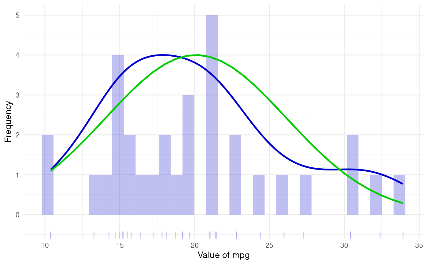
normalHist

normalHist generates a histogram with a density curve and a normal density curve.

normalHist(
  vector,
  histColor = "#0000CC",
  distributionColor = "#0000CC",
  normalColor = "#00CC00",
  distributionLineSize = 1,
  normalLineSize = 1,
  histAlpha = 0.25,
  xLabel = NULL,
  yLabel = NULL,
  normalCurve = TRUE,
  distCurve = TRUE,
  breaks = 30,
  theme = ggplot2::theme_minimal(),
  rug = NULL,
  jitteredRug = TRUE,
  rugSides = "b",
  rugAlpha = 0.2,
  returnPlotOnly = FALSE
)

# S3 method for normalHist
print(x, ...)

Arguments

vector

A numeric vector.

histColor

The colour to use for the histogram.

distributionColor

The colour to use for the density curve.

normalColor

The colour to use for the normal curve.

distributionLineSize

The line size to use for the distribution density curve.

normalLineSize

The line size to use for the normal curve.

histAlpha

Alpha value ('opaqueness', as in, versus transparency) of the histogram.

xLabel

Label to use on x axis.

yLabel

Label to use on y axis.

normalCurve

Whether to display the normal curve.

distCurve

Whether to display the curve showing the distribution of the observed data.

breaks

The number of breaks to use (this is equal to the number of bins minus one, or in other words, to the number of bars minus one).

theme

The theme to use.

rug

Whether to add a rug (i.e. lines at the bottom that correspond to individual datapoints.

jitteredRug

Whether to jitter the rug (useful for variables with several datapoints sharing the same value.

rugSides

This is useful when the histogram will be rotated; for example, this can be set to 'r' if the histogram is rotated 270 degrees.

rugAlpha

Alpha value to use for the rug. When there is a lot of overlap, this can help get an idea of the number of datapoints at 'popular' values.

returnPlotOnly

Whether to return the usual normalHist object that also contains all settings and intermediate objects, or whether to only return the ggplot2::ggplot() plot.

x

The object to print.

...

Any additional arguments are passed to the default print method.

Value

An object, with the following elements:

input

The input when the function was called.

intermediate

The intermediate numbers and distributions.

dat

The dataframe used to generate the plot.

plot

The histogram.

Author

Gjalt-Jorn Peters

Maintainer: Gjalt-Jorn Peters gjalt-jorn@userfriendlyscience.com

Examples

normalHist(mtcars$mpg)