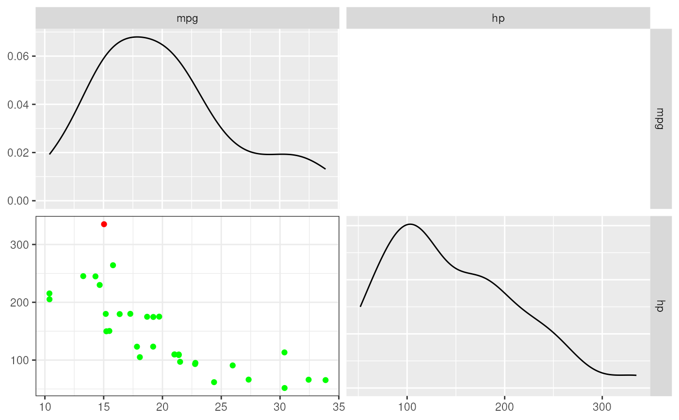
This function combines a number of criteria for determining whether a datapoint is an influential case in a regression analysis. It then sum the criteria to compute an index of influentiality. A list of cases with an index of influentiality of 1 or more is then displayed, after which the regression analysis is repeated without those influantial cases. A scattermatrix is also displayed, showing the density curves of each variable, and in the scattermatrix, points that are colored depending on how influential each case is.
regrInfluential(formula, data, createPlot = TRUE)

# S3 method for regrInfluential
print(x, headingLevel = 3, ...)
Arguments
- formula
The formule of the regression analysis.
- data
The data to use for the analysis.
- createPlot
Whether to create the scattermatrix (requires the
GGallypackage to be installed).- x
Object to print.
- headingLevel
The number of hash symbols to prepend to the heading.
- ...
Additional arguments are passed on to the
regrprint function.
Value
A regrInfluential object, which, if printed, shows the
influential cases, the regression analyses repeated without those cases, and
the scatter matrix.
Examples
regrInfluential(mpg ~ hp, mtcars);
#>
#> ### Influential cases:
#>
#>               mpg  hp    dfb.1_   dfb.hp    dffit     cov.r   cook.d       hat
#> Maserati Bora  15 335 -1.128627 1.487575 1.580208 0.9791369 1.052231 0.2745929
#>               indexOfInfluentiality
#> Maserati Bora                     5

#>
#> #### Regression analyses, repeated without influential cases
#>
#>
#> ##### Omitting all cases marked as influential by 5 criteria
#>
#> Regression analysis for formula: mpg ~ hp
#>
#> Significance test of the entire model (all predictors together):
#>   Multiple R-squared: [0.41, 0.79] (point estimate = 0.6, adjusted = 0.59)
#>   Test for significance: F[1, 30] = 45.46, p < .001
#>
#> Raw regression coefficients (unstandardized beta values, called 'B' in SPSS):
#>
#>             95% conf. int. estimate   se     t     p
#> (Intercept) [26.76; 33.44]    30.10 1.63 18.42 <.001
#> hp          [-0.09; -0.05]    -0.07 0.01 -6.74 <.001
#>
#> Scaled regression coefficients (standardized beta values, called 'Beta' in SPSS):
#>
#>             95% conf. int. estimate   se     t     p
#> (Intercept)  [-0.23; 0.23]     0.00 0.11  0.00     1
#> hp          [-1.01; -0.54]    -0.78 0.12 -6.74 <.001
#>
#> #### Regression analyses, repeated without influential cases
#>
#>
#> ##### Omitting all cases marked as influential by 5 criteria
#>
#> Regression analysis for formula: mpg ~ hp
#>
#> Significance test of the entire model (all predictors together):
#> Multiple R-squared: [0.41, 0.79] (point estimate = 0.6, adjusted = 0.59)
#> Test for significance: F[1, 30] = 45.46, p < .001
#>
#> Raw regression coefficients (unstandardized beta values, called 'B' in SPSS):
#>
#> 95% conf. int. estimate se t p
#> (Intercept) [26.76; 33.44] 30.10 1.63 18.42 <.001
#> hp [-0.09; -0.05] -0.07 0.01 -6.74 <.001
#>
#> Scaled regression coefficients (standardized beta values, called 'Beta' in SPSS):
#>
#> 95% conf. int. estimate se t p
#> (Intercept) [-0.23; 0.23] 0.00 0.11 0.00 1
#> hp [-1.01; -0.54] -0.78 0.12 -6.74 <.001